


|
Navigation: Toolboxes > Control Toolbox > MLP Network Editor > Introduction to MLP Networks |
  
|
The basic element of the Multi Layer Perceptron (MLP) neural network, is the artificial neuron. An artificial neuron, is a unit that performs a simple mathematical operation on its inputs. In the figure below, the neuron is graphically presented.
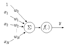
The input, x, of the neuron consists of the variables x1 ... xn and a bias term, known as the momentum constant, which is equal to 1. Each of the input values is multiplied by a weight, wi , after which the results are added. On the result, a simple mathematical function, f (x), is performed. This function is also known as the activation function. The calculations the neuron performs are thus given by:
y = f ( w0 + x1*w1 + ... + xn*wn )
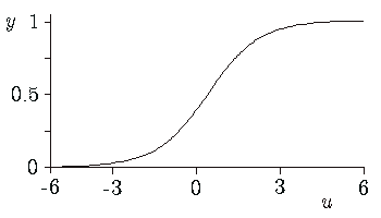
Numerous choices for the functions exist. Frequently used implementations are the Sigmoid functions:
f(u) = 1 / (1 + e-u )
f (u) = c1 * tanh ( c2 * u)
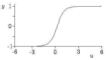
(in the picture c1 = c2 = 1)
An MLP network, as any type of back-propagation network can consist of many neurons, which are ordered in layers. The neurons in the hidden layers do the actual processing, while the neurons in the input and output layer merely distribute and collect the signals. Although many hidden layers can be used, it has been shown that an MLP with one hidden layer can approximate any continuous function. Therefore in 20-sim, the MLP networks only have one hidden layer.
The MLP network is trained by adapting the weights. During training the network output is compared with a desired output. The error between these two signals is used to adapt the weights. This rate of adaptation is controlled by the learning rate. A high learning rate will make the network adapt its weights quickly, but will make it potentially unstable. Setting the learning rate to zero, will make the network keep its weights constant.