Navigation:  Editor > Compiling > Integral Form

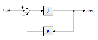
Consider the following first order linear model:

This model can be described by the dynamic equation:

 

output = int( input - K*output )

 

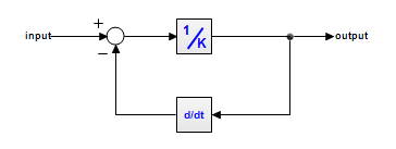
Now look at the following model:

This model can be described by the dynamic equation:

 

output = ( input - ddt(output) )/K

 

Note that we can rewrite this equation as:

 

ddt(output) = input - K*output

 

or

 

output = int( input - K*output )

 

This is the same equation as the previous model! Apparently, both models are the same! Both models can therefore be described by the dynamic equations:

 

ddt(output) = input - K*output

output = int( input - K*output )

 

We call the first equation the differential form (no integrals). The second equation is called the integral form (no derivatives). In 20-sim, models can be entered in integral form as well as the differential form.

Solving Differential Equations

During compilation, 20-sim will automatically try to rewrite equations into the integral form, since this leads to more efficient simulation. Sometimes an integral form cannot be found. Then algorithms will be applied to solve the differential directly. For example an equation like:

 

output = ddt(sin(a*time))

 

will be replaced by the following equation (applying the chain rule and using the known derivative for the sine function):

 

output = a*cos(a*time)

 

Sometimes a differential cannot be solved directly. Then only the Backward-Differentiation Methods can be used for simulation.

Simulation Code

After compilation simulation code is generated. The equation in integral form:

 

output = int( input - K*output )

 

will be written as:

 

independent state = output

independent rate = input - K*output

 

and can be handled by all integration methods. The equation in differential form:

 

ddt(output) = input - K*output

 

will be written as:

 

dependent rate = input - K*output

dependent state = output

 

and can only be handled by the Backward-Differentiation Methods.