Bond Graph
Domains: Continuous. Size: 1-D. Kind: Bond Graphs.
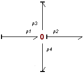
This junction is equal to a normal zero junction but monitors the powerflows through the connected bonds. If you use this junction and connect some bonds, it could look like the figure below. The bond numbers are important for identification. You can see them by clicking Port Names from the View menu.

The constitutive equations for this example are:
p1.f - p2.f - p3.f - p4.f = 0;
p1.e = p2.e = p3.e = p4.e;
output = p2.e;
The powerflows through the junction are monitored:
power = p.e .* p.f;
Note that power is a vector with a size equal to the number of bonds that are attached to the junction. The first element of the vector is the power of the first bond (p1 in the example figure), the second element is the power of the second bond (p2 in the example figure) and so on. To see which bonds are active and which bonds are not, the activity is calculated:
activity = int (abs (power));
To get an easy comparison, the relative activity is calculated:
maximum_activity = max (activity);
relative_activity = activity ./ maximum_activity
Ports |
Description |
p[any] |
Any number of ports may be connected. |
Causality |
|
1_flow p |
Only one port may have a flow out causality (as seen from the element). |
Outputs |
|
effort |
The output signal is equal to the effort of the ports. |
Variables |
|
power |
Vector of which the elements are the powers of the connected bonds. |
activity |
Vector of which the elements are the integrated absolute powers of the connected bonds. |
relative_activity |
Vector of which the elements are the relative activities of the connected bonds. |
All connected bonds must have size 1.


