


Line |
  
|
Iconic Diagrams\Hydraulics\Components
Domains: Continuous. Size: 1-D. Kind: Iconic Diagrams (Hydraulics).
The line model represents a hydraulic pipe or hose with elasticity, inertia and pressure drop. It is assumed that the pipe or hose is round and has a certain length. The line model has two implementations: Default and MultipleCells.
The default model of a line consists of two volumes for the compressibility of the fluid, a hydraulic inertia for the mass of the fluid and a friction element to model to friction of the fluid with the walls.
The default line model contains the smallest number of elements to correctly represent the behaviour of a hydraulic line. A more detailed model is obtained by repeating these elements in cells. The more cells are used, the more detailed the fluid flow inside the line can be simulated.
In general, the default line model will do fine for modelling hydraulic circuits. Only if long lines are used and the resonances, inside the line are important, the multiple cells line model should be applied.
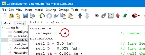
| 1. | Select the Line model in the 20-sim Editor |
| 2. | Make sure it has the MultipleCells implementation: select Right mouse menu – Edit Implementation – MultipleCells. |
| 3. | Click Go Down to inspect the equations. |
| 4. | Change the value of the constant n from 4 to the number of cells that you require (n>1). |
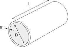
The pipe with length L [m], diameter D [m] and thickness th [m] will expand under if a pressure is applied by the fluid flowing in the pipe.
The expansion is modelled in the radial direction (pipe wall expanding) and in the length of of the pipe (pipe extending). This expansion can be modelled by a reduction of the Bulk modulus:
p = B*int(Q/V) with B = 4*th*E*B / (4*th*E + 5*D*B)
where E is Young’s modulus [Pa].
The fluid in the pipe will oppose any change in velocity by a pressure drop. This is modelled by a hydraulic inertia. The equation for the inertia is:
Q = A/(rho*L)
where A is the pipe cross sectional area [m2] and rho is the fluid density [kg/m3].
Any fluid flowing through a pipe will experience friction resulting in a pressure drop. The pressure drop depends on the fluid velocity and flow conditions. The flow condition can be determined by the Reynolds number:
Re = Q*D/(A*kv)
where Q is the fluid flow [m3/s], D the pipe diameter [m], A the pipe cross sectional area [m2] and kv the kinematic viscosity [m2/s].
For low Reynolds numbers the flow is laminar and for high Reynolds numbers the flow is turbulent. According to Beater (1999), for a smooth pipe, the friction factor lambda can be described as:
lambda = 2*dp*D/(v^2*rho*L)
with dp the pressure drop [Pa] over the line, rho the density of the fluid [kg/m3] and v the average flow velocity of the fluid.
The friction factor lambda depends on the Reynolds number:
Re |
lambda |
flow |
0 - 1404 |
64/Re |
laminar (Hagen=Poiseuille) |
1404-2320 |
0.0456 |
transition from laminar to turbulent |
> 2320 |
0.3164 / Re0.25 |
turbulent (Blasius) |
Ports |
Description |
pa, pb |
Both terminals of the hydraulic inertia. |
Causality |
|
fixed pressure out pa fixed pressure out pb |
|
Parameters |
|
D L th E |
Line inner diameter [m] Line length [m] Wall thickness [m] Modulus of elasticity [N/m2] |