An adaptive B-spline network can be used to relate k inputs and a single output y on a restricted domain of the input space. The following network shows a realization with one input:
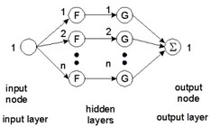
The network is shown with two hidden layers. Some authors prefer to show a B-spline network with only one hidden layer. For a proper understanding of multi-dimensional B-spline networks we prefer to show the network with two hidden layers.
The first hidden layer distributes the inputs over several nodes. In the figure above input 1 is distributed over n nodes. Each node of this layer has only one input. To this input a "basis function" F is applied. As basis functions, B-splines are used of any desired order. An N-th order B-spline function consists of pieces of (N-1)th order polynomials, such that the resulting function is (N-1) times differentiable. The figure below shows examples of B-spline functions of different order. A spline function differs from zero on a finite interval.
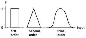
The second hidden layer also consists of n nodes. Each node of this layer has only one input. To this input a function G is applied which is merely a multiplication by a weight:
G = w * i
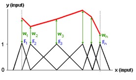
The output node sums the results of all second hidden layer nodes. When the spline functions of the various nodes are properly spaced, every one dimensional function can be approximated. This is shown in the figure below where the various splines (F1 to Fn) combined with the various weights (w1 to wn), together form an output function.
Two-dimensional B-spline networks have two input nodes. The first hidden layer, as with the one-dimensional network, consists of nodes, to which a basis function F is applied. This is shown in the figure below. To the first input a group of n nodes are applied, and to the second input a group of m nodes are applied.

The second hidden layer now consists of nodes which each have two inputs. For every combination of a node from one group and and a node from the second group, a node exists. To each node of the second hidden layer, a function G is applied which is merely a multiplication of the two inputs multiplied by a weight:
G = w * i1 * i2
Again the output node sums the results of all second hidden layer nodes. When the spline functions of the various nodes are properly spaced, every two dimensional function can be approximated. The figure below shows the spacing of various spline functions of the two inputs and one output of a node of the second hidden layer.
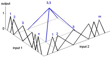
The output node sums the results of all second hidden layer nodes. When the spline functions of the various nodes are properly spaced, every two dimensional function can be approximated. This is shown in the figure below.
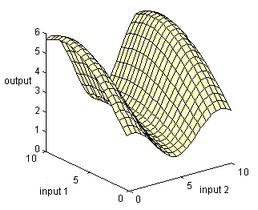
In a same way more dimensional B-spline networks can be created, using more inputs. The 20-sim B-spline Editor supports networks with up to 256 inputs and one output.
The B-spline network is trained by adapting the weights. During training the network output is compared with a desired output. The error between these two signals is used to adapt the weights. This rate of adaptation is controlled by the learning rate. A high learning rate will make the network adapt its weights quickly, but will make it potentially unstable. Setting the learning rate to zero, will make the network keep its weights constant. Learning of B-spline networks can either be done after each sample (learn at each sample), or after series of samples (learn after leaving spline).
When learning at each sample, after every sample the weights are adapted according to:
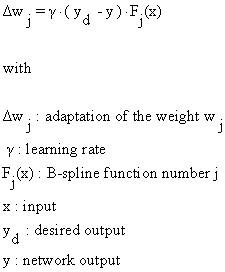
Given a certain input (x), only a limited number of splines Fi (x) are nonzero. Therefore only a few weights are adapted each sample.
When learning after leaving a spline, the network will keep track of the input (x) and the corresponding nonzero splines Fi (x). For each nonzero spline, a sample will be stored consisting of the input (x), the output (y) and desired output (yd). Only after the input has left the region where a spline is nonzero, its weight is updated according to:

Here n is the number of samples that have been taken.