


|
Navigation: Toolboxes > Control Toolbox > Controller Design Editor > Transfer Functions |
  
|
A continuous time or discrete time SISO transfer function:
|
|
(continuous) |
(discrete) |
is characterized by its numerator n and denominator d, both polynomials of the variable s or z.

You can enter transfer functions by selecting the Transfer Function button and clicking the Edit button.
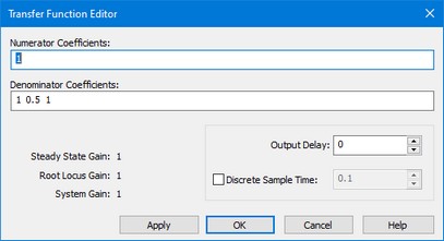
This opens an editor in which you can enter the coefficients of the numerator and denominator polynomials. You can enter the elements in the white space areas. Separate the elements with Spaces. Polynomials should be entered in descending powers of s or z. The Steady State Gain, Root Locus Gain and System Gain are parameters, that are automatically derived from the transfer function.
In the editor shown above the transfer function
![]()
was given. You can enter the coefficients as:
1
and
1 0.5 1
or
0.1,0.1
and
1,1,0.5
To inspect the effects of time delay in your model, you can add output delay. The result will be visible in the various plots that you can show of a linear system. The unit of the output delay is seconds.
If you want to transfer a linear system from continuous time to discrete time directly (i.e. replace the s by a z), select Discrete Sample time and fill in the sample time value. You can also transfer back directly by deselecting Discrete Sample time.
| • | Help: Open the help file. |
| • | Apply: Apply the current changes of the system, recalculate each plot that is active (step, Bode, Nyquist, Nichols, pole zero). |
| • | OK: Apply the current changes of the system, recalculate each plot that is active (step, Bode, Nyquist, Nichols, pole zero) and close the editor. |
| • | Cancel: Do not apply any changes to the system and close the editor. |