


|
Navigation: Toolboxes > Frequency Domain Toolbox > Dynamic Error Budgeting > Dynamic Error Budgeting |
  
|
The performance of precision machines is mostly limited by the disturbances that are injected in these machines. These disturbances are often stochastic in nature. Dynamic Error Budgeting is a method whereby the effect of these disturbances on the final performance can be calculated. The advantage of this method is that it enables the designer to enter the contributions of the individual disturbances and view and optimize the overall machine performance.
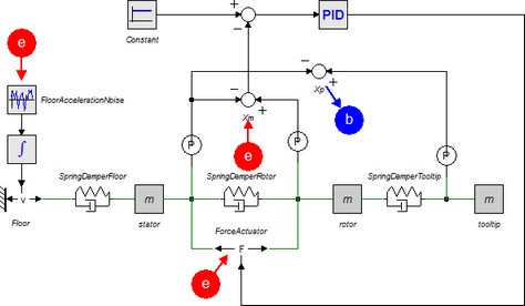
The Dynamic Error Budgeting toolbox shows the total error as a result of injected disturbances.
| 1. | Open the example model Dynamic Error Budgetting from the Getting Started/Frequency Domain Toolbox. |
You can open the Dynamic Error Budgeting tool in the Simulator:
| 2. | From the Tools menu select Frequency Domain Toolbox and Dynamic Error Budgeting. |
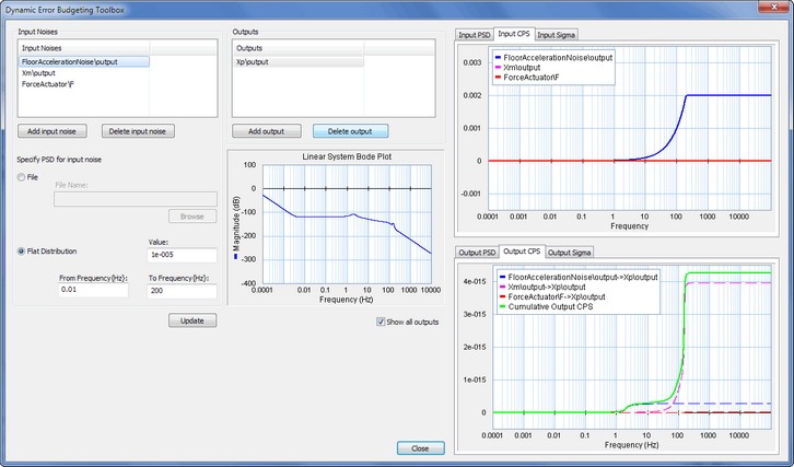
The Dynamic Error Budgeting tool.
The tool allows you to enter disturbances (as power spectral density) in the Input Noises section.
| 3. | For each disturbance you have to select a corresponding variable by clicking the Add input noise button. |
Each disturbance is effectively a summation to the chosen variable, just like closed loop linearization. You can inspect each disturbance in the graph on the top right.
Next you have to select an output variable, where the result of the disturbances is calculated.
| 4. | Select the output by clicking the Add Output button. |
In the graph on the bottom right you can see the resulting error at the selected output as a result of the disturbances. The error is given in the form of a power spectral density (PSD) and cumulative power spectral density (CPS). The square root of the final value of the CPS is equal to the standard deviation of the output error. The standard deviations are shown in the Output Sigma tab.