
Frequency Domain
Frequency Domain consists of the linear system editor, FFT analysis tools, model linearization functionality and Dynamic Error Budgeting.
Linear System Editor
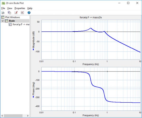
The Linear System Editor is a specialized tool for the design and analysis of linear systems. The editor supports continuous-time and discrete-time SISO systems using various representations. The graphical interface allows you to edit a linear system in any desired form: ABCD state space, Transfer Function or Zero Pole Gain. Analyzing the Step response, Bode plot, Nyquist diagram, Nichols chart and Pole-Zero plots allows you to quickly evaluate system behavior.
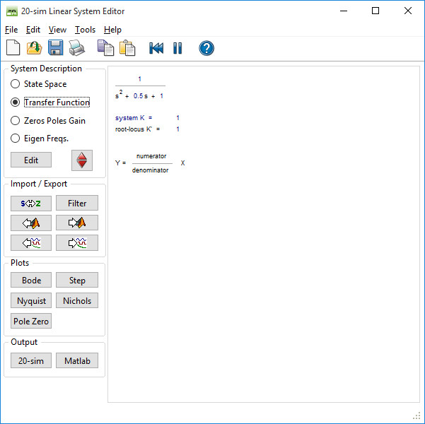
Phase, gain and modulus margins are calculated, as well as rise time, overshoot and steady state value. Input can originate from a 20-sim linear system model, 20-sim filter or control editor, MATLAB workspace, or user input. You are able to generate output for all 20-sim editors, the clipboard and the MATLAB workspace.
Fast Fourier Transform
Fast Fourier Transforms (FFT) can be applied to any time-domain plot in 20-sim. Either simulation results or measurement data will do. When the data is not equally spaced, linear interpolation is first applied after which the Fast Fourier Transform is used to calculate the frequency contents. Three representations are supported: Amplitude and Phase plot, Frequency plot and Power Spectral Density plot.
Linearization
Any 20-sim model can be linearized to state space form. If possible, linearization will be performed symbolically. Otherwise linearization will be performed numerically. The resulting state space model is shown in the 20-sim Linear System Editor. The Linear System Editor is a specialized tool for the design and analysis of linear systems. The editor supports continuous-time and discrete-time SISO systems using various representations. Standardized plots enable you to quickly evaluate system behavior. If possible, any 20-sim model can be linearized.
Features
- Editing as ABCD state space, Transfer Function or Zero Pole Gain with automatic transformation between these forms.
- Transfer between continuous-time and discrete-time representation.
- View characteristic properties like eigenfrequencies and damping.
- Handles numeric and symbolic models.
- Various plot options: Step Response, Bode Plot, Nyquist Diagram, Nichols Chart and Pole-Zero Plot.
Dynamic Error Budgeting
Dynamic Error Budgeting is a method whereby the effect of disturbances on the final performance of a system can be calculated. 20-sim has a special tool make Dynamic Error Budgeting straightforward and simple.