
Introduction to 20-sim
20-sim is a modeling and simulation software package for mechatronic systems. It runs on PC-computers with a Windows OS (Vista, 7, 8, 8.1 and 10) and requires 450 MB of disk space. With 20-sim, models can be created graphically, similar to drawing an engineering scheme. With these models, the behaviour of dynamic systems can be analyzed and control systems can be designed. 20-sim models can be exported as C-code to be run on hardware for rapid prototyping and HIL-simulation.
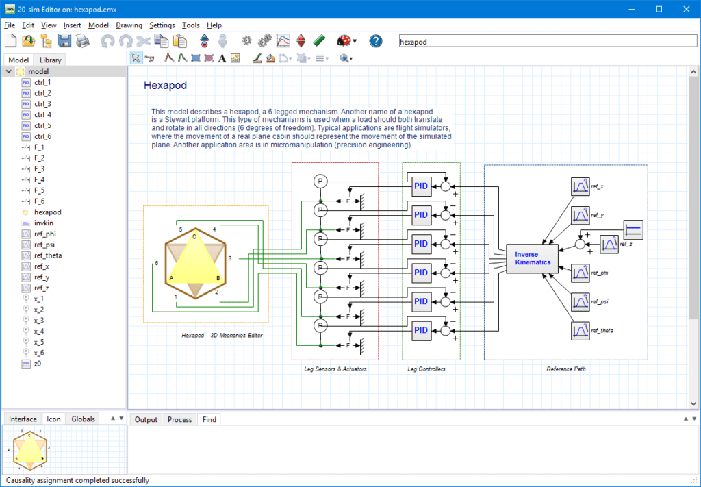
The image above shows 20-sim with a model of a controlled hexapod. The mechanism is generated with the 3D mechanics feature and connected with standard actuator and sensor models from the mechanics library. The hexapod is controlled by PID controllers which are tuned in the frequency domain. Everything that is required to build and simulate this model is inside the package. No external software or compiler is needed! This article gives a small introduction to 20-sim.
Editor
The 20-sim software consist of 2 windows which are tightly integrated. Models are created in the editor and simulation runs and results are shown in the simulator. When 20-sim is started, the editor will open. The editor contains a model library tree from which you can drag and drop elements to the drawing canvas to construct your models. The 20-sim editor will display as a graphical editor or a text editor depending on the model that is shown. The library contains elements for building bond graph models, components for building physical systems and blocks for building block diagram models. All library elements are open and can be changed by the user. The library contains the following elements:
- Bond Graph: Elements for building bond graph models.
- Iconic Diagrams: Components for building physical systems.
- Electric: Components for building electric networks.
- Mechanical: Components for building translational and rotational mechanical structures.
- Hydraulics: Components for building hydraulic systems.
- Thermal: Components for modelling heat transfer.
- Block Diagrams: Blocks for building block diagram models: Linear and non-linear blocks, sources & sinks, transfer functions.
- Examples: Example models showing the basic use of the library models.
Graphical Models
Models in 20-sim are hierarchically oriented. The model on top is called the main model. It is constructed out of graphical elements which are called submodels. Submodels can be easily connected. Depending on the submodel, the connection can be a shared variable or a physical connection. A submodel itself can be constructed from multiple submodels, and these submodels themselves can be constructed with submodels, going many layers deep. At the bottom of the hierarchy, the models are described by sets of equations. These models are called equation models.
Equation Models
Equation models are specified in a special language called SIDOPS++. SIDOPS++ has great resemblance with Maple, Matlab and other mathematical software packages.
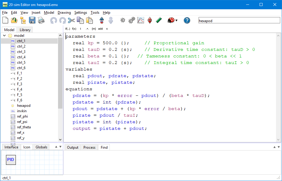
The picture above shows an example of an equation model. 20-sim equation models have a basic layout indicated by keywords
Parameters: Definition of values, that do not change during simulation.
Variables: Definition of values that do change during simulation.
Equations: The actual equations.
Equations are relations between parameters and variables and indicated by an equal (=) sign. Various mathematical functions and operators are available for use in equations.
Modeling Tools
20-sim comes with a number of features to build advanced models:
- Controller Design Editor: This feature helps users to design feedback systems with a linear plant, controller and pre-filter. Open and closed loop responses can be investigated using Bode and Nyquist plots.
- 3D Mechanics Editor: 3D mechanical systems are notoriously difficult to model using 1D elements. Therefore, the 3D Mechanics Editor enables the user to define mechanical systems by dragging and dropping bodies, joints and other objects in a 3D workspace. The corresponding set of optimized differential equations is generated automatically.
- Wizards: Various wizards will help you to create motion profiles, define cams, build servo motors and much more.
Simulation
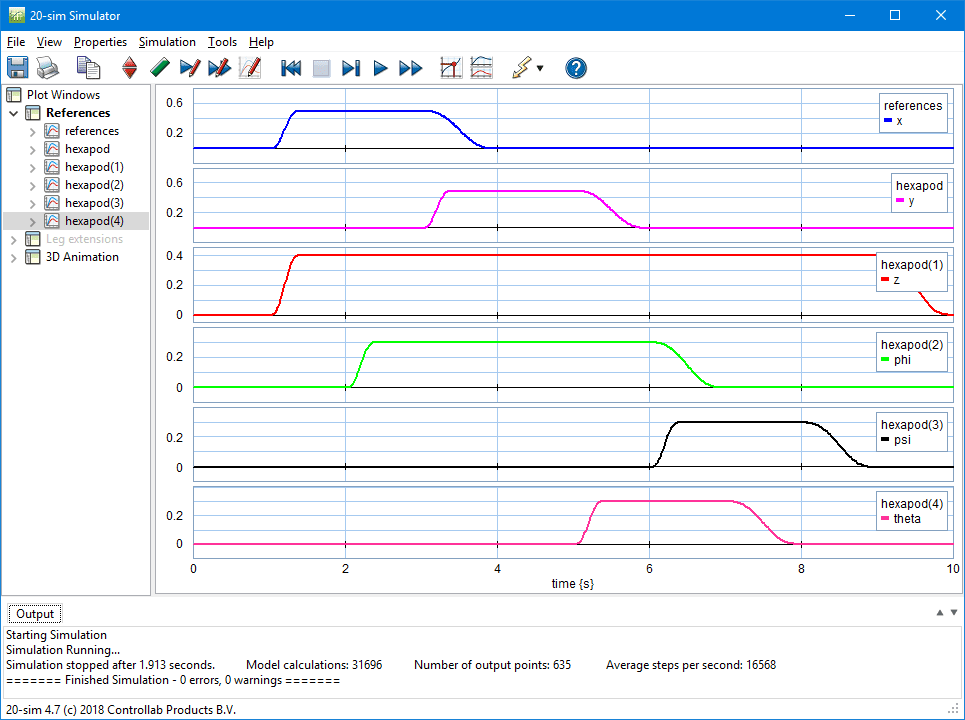
When a model is ready, the simulator can be opened from the editor. Under the hood, the model is automatically compiled to create simulation code. No external tools are required. In the compiling-phase, 20-sim will check if the model is correct and optimize the equations. The simulator is used to run simulations and analyze models. Before a simulation run can be started, the user has to define some settings:
- Run properties: The start time and finish time of a run.
- Integration method: 20-sim supports a number of advanced numerical methods for running a simulation. The numerical method can be chosen along with proper settings. These settings include for example maximum integration error and step size.
- Parameter values: Before a simulation run, the default parameters values may have to be changed.
- Plot properties: The number and appearance of the plots have to be set and the variables to be plotted have to be chosen.
Next to simulation plots, results can also be shown as 3D animations in 20-sim. A special editor is available in which any variable can be connected to the position, orientation, size and colour of 3D objects. Standard 3D objects are available like cubes and spheres but objects can also be imported from CAD packages.
Analysis
The 20-sim package has two features which can be used to analyze models.
- Time Domain: This allows model analysis by changing parameters values and using multiple simulation runs. Parameter sweeps, Optimization and Curve Fitting will help to improve the system performance. Sensitivity Analysis, Monte Carlo Analysis and Variation Analysis, will help to check the robustness of a system.
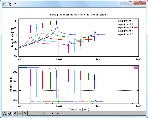
- Frequency Domain: Models in 20-sim can be linearised to show the corresponding linear system in the Linear System Editor. The Linear System Editor is a specialized tool for the design and display of linear systems. The editor supports continuous-time and discrete-time SISO systems and can show the system response by bode and Nyquist plots. If models cannot be linearised, Fast Fourier Transforms can be used to show the frequency behaviour of a model.
Scripting
With scripting, tasks can be run in 20-sim automatically using specialized scripting functions. With these functions models can be opened and run automatically, parameters can be changed, results can be exported and much more.
20-sim scripting functions can be run as m-files in Matlab or GNU Octave. GNU Octave is an open source environment that allows to run m-files similar to Matlab. Scripting functions are available to open and simulate 20-sim models, export parameters values to a 20-sim model, run simulations, export simulation plots and much more.
Code Generation
Out of any 20-sim model, C-code can be generated for use in external systems, HIL simulators etc. Templates allow customization of the C-code with pre and post commands, file-linking, comments etc. There are built-in templates that allow you to generate code for various targets:
- 20-sim 4C: The package 20-sim 4C helps to run C-code on hardware to control machines and systems. 20-sim 4C imports models (c-code) from 20-sim and runs them on hardware like embedded arm boards, PC 104 systems and much more. For more information, see www.20sim4c.com.
- Matlab Simulink: Generating C-code for use in MATLAB Simulink also includes a submodel block with input and output terminals. 20-sim uses the MEX-compiler, to compile this code directly into an S-function. These S-functions can also be used in the Real Time Workshop in order to generate code for a specific platform, for instance xPC Targets.
- C-Code: 20-sim can generate stand-alone C-code for use in C and C++ programs. The generated C-code is supplied with several fixed step simulation algorithms to enable it to run in real-time. The Euler and Runge-Kutta methods are supported by default.